一、平穩(wěn)序列建模步驟

假如某個觀察值序列通過序列預(yù)處理可以判定為平穩(wěn)非白噪聲序列，就可以利用ARMA模型對該序列進(jìn)行建模。建模的基本步驟如下：

（1）求出該觀察值序列的樣本自相關(guān)系數(shù)（ACF）和樣本偏自相關(guān)系數(shù)（PACF）的值。

（2）根據(jù)樣本自相關(guān)系數(shù)和偏自相關(guān)系數(shù)的性質(zhì)，選擇適當(dāng)?shù)腁RMA（p，q）模型進(jìn)行擬合。

（3）估計模型中位置參數(shù)的值。

（4）檢驗(yàn)?zāi)Ｐ偷挠行浴Ｈ绻Ｐ筒煌ㄟ^檢驗(yàn)，轉(zhuǎn)向步驟（2），重新選擇模型再擬合。

（5）模型優(yōu)化。如果擬合模型通過檢驗(yàn)，仍然轉(zhuǎn)向不走（2），充分考慮各種情況，建立多個擬合模型，從所有通過檢驗(yàn)的擬合模型中選擇最優(yōu)模型。

（6）利用擬合模型，預(yù)測序列的將來走勢。

二、代碼實(shí)現(xiàn)

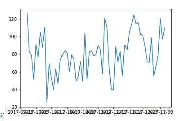
1、繪制時序圖，查看數(shù)據(jù)的大概分布

trainSeting.head()Out[36]: date2017-10-01 126.42017-10-02 82.42017-10-03 78.12017-10-04 51.12017-10-05 90.9Name: sales, dtype: float64plt.plot(trainSeting)

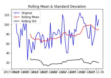
2、平穩(wěn)性檢驗(yàn)

’’’進(jìn)行ADF檢驗(yàn)adf_test的返回值Test statistic：代表檢驗(yàn)統(tǒng)計量p-value：代表p值檢驗(yàn)的概率Lags used：使用的滯后k，autolag=AIC時會自動選擇滯后Number of Observations Used：樣本數(shù)量Critical Value(5%) : 顯著性水平為5%的臨界值。(1)假設(shè)是存在單位根，即不平穩(wěn)；(2)顯著性水平，1%：嚴(yán)格拒絕原假設(shè)；5%：拒絕原假設(shè)，10%類推。(3)看P值和顯著性水平a的大小，p值越小，小于顯著性水平的話，就拒絕原假設(shè)，認(rèn)為序列是平穩(wěn)的；大于的話，不能拒絕，認(rèn)為是不平穩(wěn)的(4)看檢驗(yàn)統(tǒng)計量和臨界值，檢驗(yàn)統(tǒng)計量小于臨界值的話，就拒絕原假設(shè)，認(rèn)為序列是平穩(wěn)的；大于的話，不能拒絕，認(rèn)為是不平穩(wěn)的’’’#滾動統(tǒng)計def rolling_statistics(timeseries): #Determing rolling statistics rolmean = pd.rolling_mean(timeseries, window=12) rolstd = pd.rolling_std(timeseries, window=12) #Plot rolling statistics: orig = plt.plot(timeseries, color=’blue’,label=’Original’) mean = plt.plot(rolmean, color=’red’, label=’Rolling Mean’) std = plt.plot(rolstd, color=’black’, label = ’Rolling Std’) plt.legend(loc=’best’) plt.title(’Rolling Mean & Standard Deviation’) plt.show(block=False) ##ADF檢驗(yàn)from statsmodels.tsa.stattools import adfullerdef adf_test(timeseries): rolling_statistics(timeseries)#繪圖 print (’Results of Augment Dickey-Fuller Test:’) dftest = adfuller(timeseries, autolag=’AIC’) dfoutput = pd.Series(dftest[0:4], index=[’Test Statistic’,’p-value’,’#Lags Used’,’Number of Observations Used’]) for key,value in dftest[4].items(): dfoutput[’Critical Value (%s)’%key] = value #增加后面的顯著性水平的臨界值 print (dfoutput) adf_test(trainSeting) #從結(jié)果中可以看到p值為0.1097>0.1，不能拒絕H0,認(rèn)為該序列不是平穩(wěn)序列

返回結(jié)果如下

Results of Augment Dickey-Fuller Test:Test Statistic -5.718539e+00p-value 7.028398e-07#Lags Used 0.000000e+00Number of Observations Used 6.200000e+01Critical Value (1%) -3.540523e+00Critical Value (5%) -2.909427e+00Critical Value (10%) -2.592314e+00dtype: float64

通過上面可以看到，p值小于0.05，可以認(rèn)為該序列為平穩(wěn)時間序列。

3、白噪聲檢驗(yàn)

’’’acorr_ljungbox(x, lags=None, boxpierce=False)函數(shù)檢驗(yàn)無自相關(guān)lags為延遲期數(shù)，如果為整數(shù)，則是包含在內(nèi)的延遲期數(shù)，如果是一個列表或數(shù)組，那么所有時滯都包含在列表中最大的時滯中boxpierce為True時表示除開返回LB統(tǒng)計量還會返回Box和Pierce的Q統(tǒng)計量返回值：lbvalue:測試的統(tǒng)計量pvalue:基于卡方分布的p統(tǒng)計量bpvalue:((optionsal), float or array) ? test statistic for Box-Pierce testbppvalue:((optional), float or array) ? p-value based for Box-Pierce test on chi-square distribution’’’from statsmodels.stats.diagnostic import acorr_ljungboxdef test_stochastic(ts,lag): p_value = acorr_ljungbox(ts, lags=lag) #lags可自定義 return p_value

test_stochastic(trainSeting,[6,12])Out[62]: (array([13.28395274, 14.89281684]), array([0.03874194, 0.24735042]))

從上面的分析結(jié)果中可以看到，延遲6階的p值為0.03<0.05，因此可以拒絕原假設(shè)，認(rèn)為該序列不是白噪聲序列。

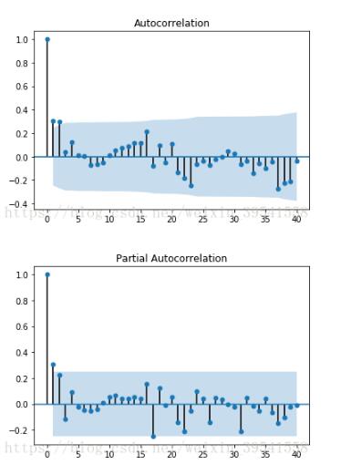
4、確定ARMA的階數(shù)

（1）利用自相關(guān)圖和偏自相關(guān)圖

####自相關(guān)圖ACF和偏相關(guān)圖PACFimport statsmodels.api as smdef acf_pacf_plot(ts_log_diff): sm.graphics.tsa.plot_acf(ts_log_diff,lags=40) #ARIMA,q sm.graphics.tsa.plot_pacf(ts_log_diff,lags=40) #ARIMA,p acf_pacf_plot(trainSeting) #查看數(shù)據(jù)的自相關(guān)圖和偏自相關(guān)圖

（2）借助AIC、BIC統(tǒng)計量自動確定

##借助AIC、BIC統(tǒng)計量自動確定from statsmodels.tsa.arima_model import ARMAdef proper_model(data_ts, maxLag): init_bic = float('inf') init_p = 0 init_q = 0 init_properModel = None for p in np.arange(maxLag): for q in np.arange(maxLag): model = ARMA(data_ts, order=(p, q)) try: results_ARMA = model.fit(disp=-1, method=’css’) except: continue bic = results_ARMA.bic if bic < init_bic: init_p = p init_q = q init_properModel = results_ARMA init_bic = bic return init_bic, init_p, init_q, init_properModel proper_model(trainSeting,40)

#在statsmodels包里還有更直接的函數(shù)：import statsmodels.tsa.stattools as storder = st.arma_order_select_ic(ts_log_diff2,max_ar=5,max_ma=5,ic=[’aic’, ’bic’, ’hqic’])order.bic_min_order’’’我們常用的是AIC準(zhǔn)則，AIC鼓勵數(shù)據(jù)擬合的優(yōu)良性但是盡量避免出現(xiàn)過度擬合(Overfitting)的情況。所以優(yōu)先考慮的模型應(yīng)是AIC值最小的那一個模型。為了控制計算量，我們限制AR最大階不超過5，MA最大階不超過5。 但是這樣帶來的壞處是可能為局部最優(yōu)。timeseries是待輸入的時間序列，是pandas.Series類型，max_ar、max_ma是p、q值的最大備選值。order.bic_min_order返回以BIC準(zhǔn)則確定的階數(shù)，是一個tuple類型

返回值如下：

order.bic_min_orderOut[13]: (1, 0)

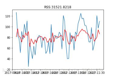
5、建模

從上述結(jié)果中可以看到，可以選擇AR(1)模型

################################模型####################################### AR模型，q=0#RSS是殘差平方和# disp為-1代表不輸出收斂過程的信息，True代表輸出from statsmodels.tsa.arima_model import ARIMAmodel = ARIMA(trainSeting,order=(1,0,0)) #第二個參數(shù)代表使用了二階差分results_AR = model.fit(disp=-1)plt.plot(trainSeting)plt.plot(results_AR.fittedvalues, color=’red’) #紅色線代表預(yù)測值plt.title(’RSS:%.4f’ % sum((results_AR.fittedvalues-trainSeting)**2))#殘差平方和

6、預(yù)測未來走勢

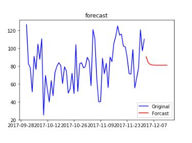
############################預(yù)測未來走勢########################################### forecast方法會自動進(jìn)行差分還原，當(dāng)然僅限于支持的1階和2階差分forecast_n = 12 #預(yù)測未來12個天走勢forecast_AR = results_AR.forecast(forecast_n)forecast_AR = forecast_AR[0]print (forecast_AR)

print (forecast_ARIMA_log)[90.49452199 84.05407353 81.92752342 81.22536496 80.99352161 80.91697003

80.89169372 80.88334782 80.88059211 80.87968222 80.87938178 80.87928258]

##將預(yù)測的數(shù)據(jù)和原來的數(shù)據(jù)繪制在一起，為了實(shí)現(xiàn)這一目的，我們需要增加數(shù)據(jù)索引，使用開源庫arrow:import arrowdef get_date_range(start, limit, level=’day’,format=’YYYY-MM-DD’): start = arrow.get(start, format) result=(list(map(lambda dt: dt.format(format) , arrow.Arrow.range(level, start,limit=limit)))) dateparse2 = lambda dates:pd.datetime.strptime(dates,’%Y-%m-%d’) return map(dateparse2, result) # 預(yù)測從2017-12-03開始，也就是我們訓(xùn)練數(shù)據(jù)最后一個數(shù)據(jù)的后一個日期new_index = get_date_range(’2017-12-03’, forecast_n)forecast_ARIMA_log = pd.Series(forecast_AR, copy=True, index=new_index)print (forecast_ARIMA_log.head())##繪圖如下plt.plot(trainSeting,label=’Original’,color=’blue’)plt.plot(forecast_ARIMA_log, label=’Forcast’,color=’red’)plt.legend(loc=’best’)plt.title(’forecast’)

以上這篇利用python實(shí)現(xiàn)平穩(wěn)時間序列的建模方式就是小編分享給大家的全部內(nèi)容了，希望能給大家一個參考，也希望大家多多支持好吧啦網(wǎng)。